Not exactly the same thing, but related: Statistical hypothesis test, p value

Comes from the stochastic nature of the input and output in machine learning.

It cannot be reduced with more training data. It can however be reduced with additional features that provide more information about the input space.

It arises from ignorance about the model due to a lack of observations.

Either there is Insufficient data. Or the model is not adequate (not complex enough) for the problem.

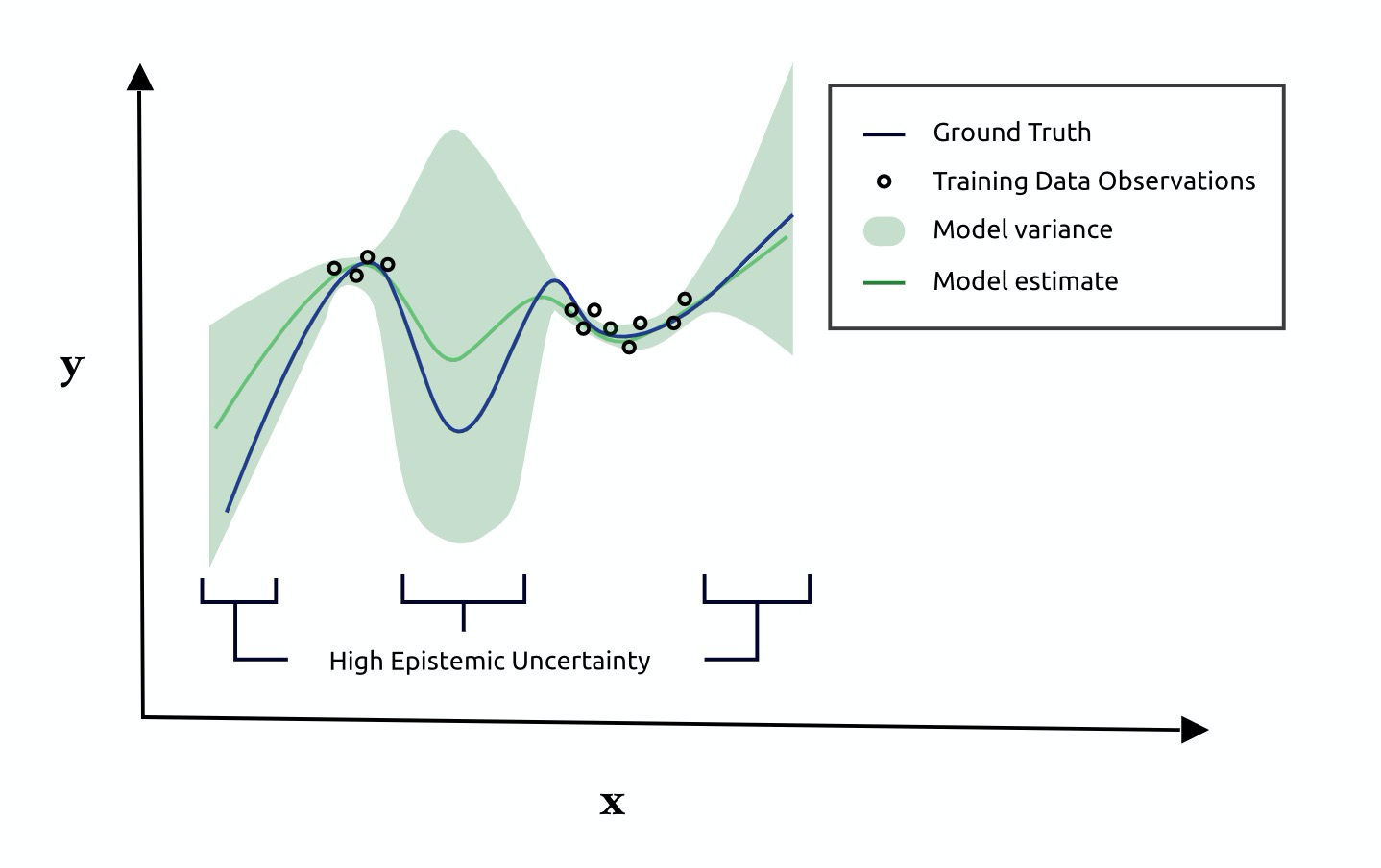
Parameter uncertainty: Limited training data (see the image above)
Model form uncertainty: Uncertainty from the model choice.

Bayesian Neural networks are an example that give as output the prediction and the uncertainty of the prediction (in the form of a mean and variance)

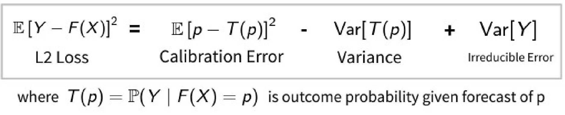
Closely related to Decomposing Model Error

Deterministic predictor: Provides a single deterministic output, ex: Linear regression
Probabilistic predictor: Outputs in the form of probability distributions, ex: Neural networks
Second order predictor: Considers uncertainty about model parameters. Ex: Bayesian neural networks.

conformal predictions.png

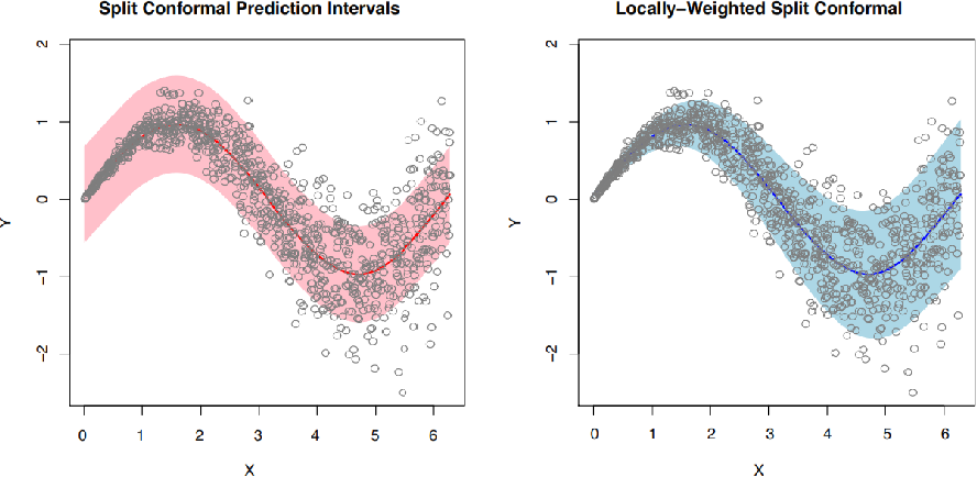
It is a framework to give certainty Intervalls. Basically the prediction will be an Intervall with a guarantee, that the result is to X percent inside of that Intervall.

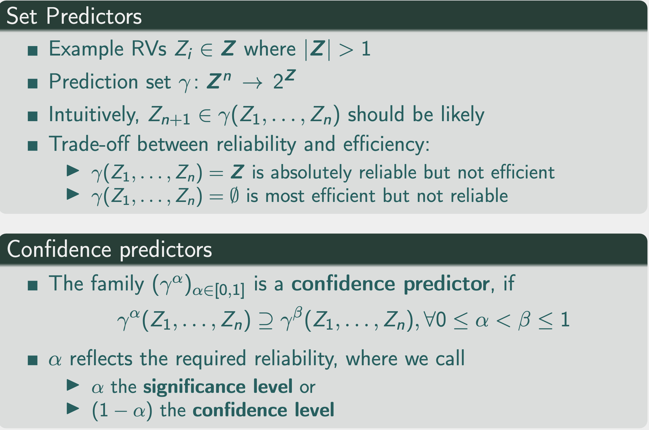
The Intervall itself can be a probability interval or even an interval of Intervalls. It is called a Set Prediction. For classification the output would be {'cat', 'dog'}, instead of just {'cat'}.

We want our conformal prediction method to have the following properties:

Efficiency: have the smallest Interval possible
Validity: Be correct
Model agnostic

The loss function can then be changed to train for better Efficiency instead of just Validity (by adding a regulating factor).

We want to calibrate our models so that the Intervalls given are as close as possible to the actual probability Intervalls.

Wrongly calibrated models are either Overconfident or Under-confident

Pasted image 20240611182532.png

We want Sharp predictions. We want the model to tell us that this person has blood pressure at 99% certainty. Not 0.5

Pasted image 20240611184522.png

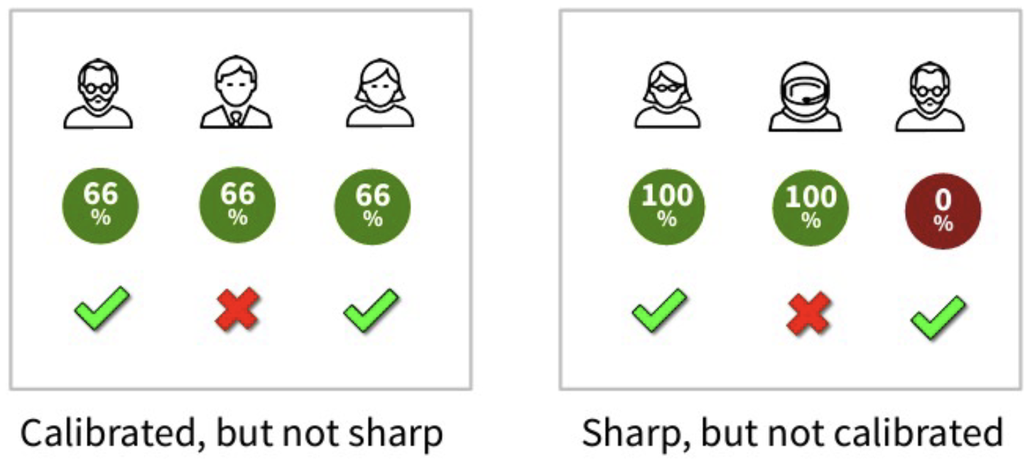
First image: 66% of predictions are correct which is true. It is calibrated. Not sharp because individual predictions are closet to 0.5 than 1 or 0.

Second image: sharp because the individual predictions are either 0 or 1. However predicting a 100% chance means that the model believes that there is a 0% chance of being wrong. Which is obviously not the case here. It is not calibrated.

Pasted image 20240614114441.png

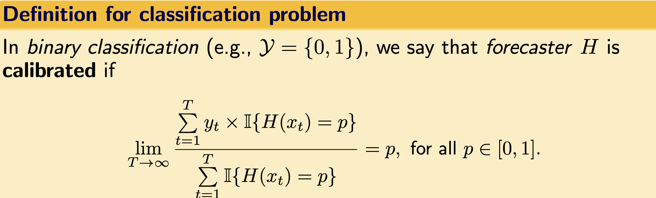
Looks complicated but its not. At an infinite amount of predictions, on average, the prediction should be as certain as it is correct.

Both approaches are not mutually exclusive

Via the Loss function

A loss function will try to:

Minimize Calibration error
Maximize sharpness

Pasted image 20240614112856.png

Via a post processing step.

Another way to fix calibration errors, is in a post processing step. Find some function, that maps the predictions onto more calibrated predictions. Computationally less expensive than to constantly tweak the loss function.

Example: Platt scaling method:

apply sigmoidal transformation to the models output whose parameters are learnt during maximum likelihood estimation.

Pasted image 20240614113658.png

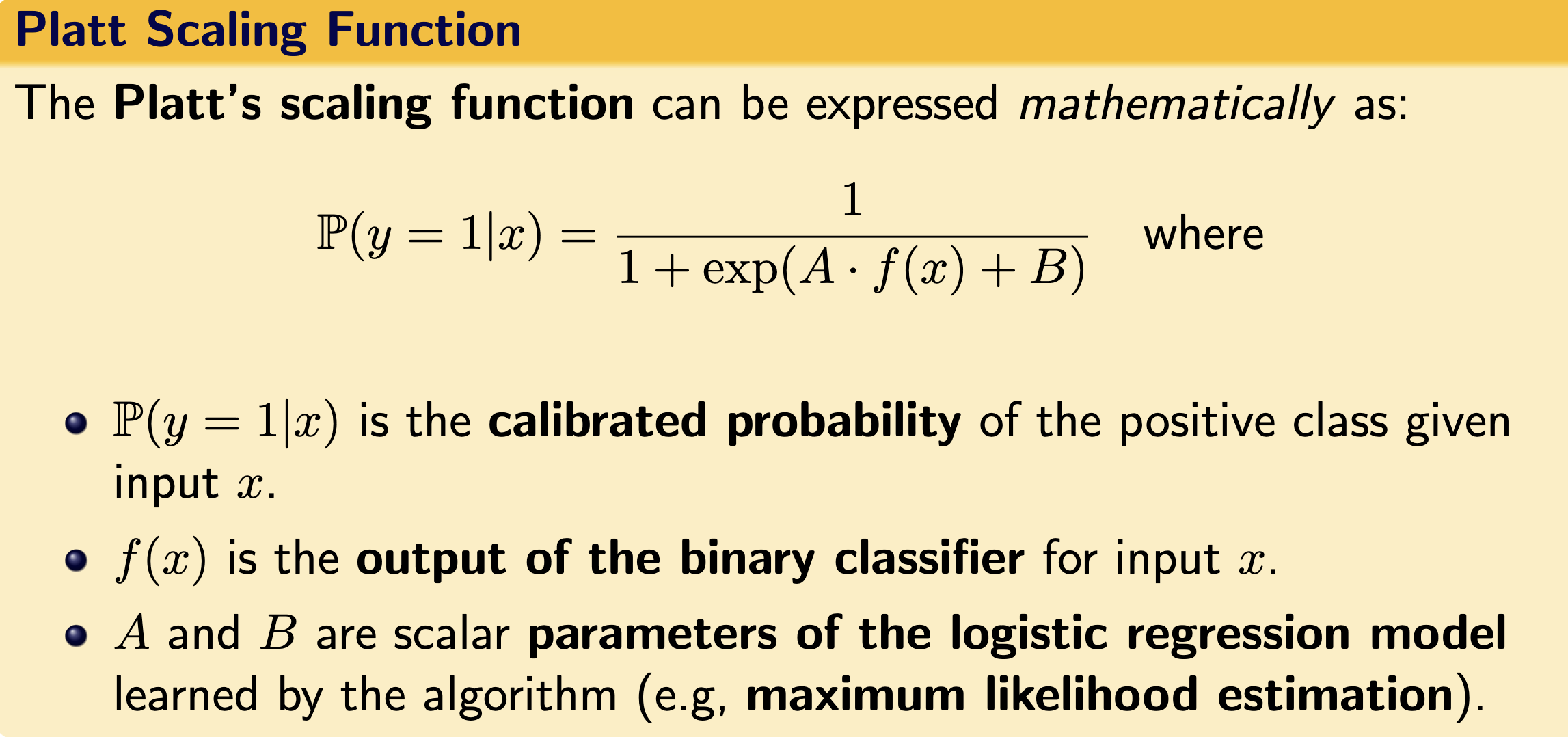
We can drive the calibration error down to zero without impacting the loss of Accuracy. "free lunch"

Piecewise affine functions

Affine function: $f (x) = A * x + b$
Piecewise Affine function:

$
\begin{equation}
f(x)=\begin{cases}
-x -5, & \text{if $x <= - 3$ }\
x + 23, & \text{if $- 3 < x <= 2$ }\
4*x + 7, & \text{if $2 < x$ }
\end{cases}
\end{equation}
$

Why Relu layers create piecewise affine function

Linear layers: $f (x) = w * x + b$ , simply an affine function
Relu Layers:
$
f(x) = \begin{cases}
0, & \text{if $x < 0$ }\
x& \text{otherwise}\
\end{cases}
$

Therefore a ReLU neural network is simply an affine function with a high number of "pieces".

Why Piece-wise affine functions are always overconfident if far away from the data.

If you move far away into one direction, at some point you will stay in a linear space until infinity (following that direction). Therefore at some point you will approach either 0 or 100% class probability, therefore 100% confidence in your prediction.

Pasted image 20240620154729.png

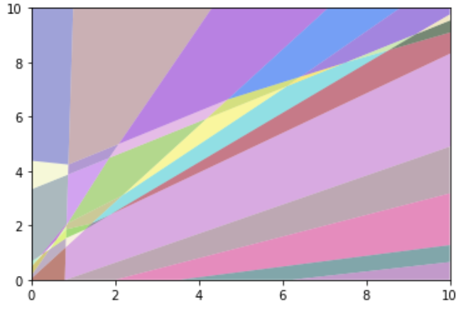
The coloured areas are the affine parts. Ignore the white dotted lines.

Why this cannot be fixed with temperature scaling.

Temperature scaling is a post processing technique to make neural networks calibrated. It divides the the logits vector (neural network output) by a learnt scalar parameter. Since our theory is valid for any $ϵ > 0$ , dividing by a scalar does not fix the problem.

Why this cannot be fixed with Softmax:

$σ (z)_{i} = \frac{e^{z_{i}}}{\sum_{j = 1}^{K} e^{z_{j}}}$
This does not change the relative magnitude of the logits. So if the original distribution is heavily skewed, then the softmax distribution will be as well.

How to fix it?

One idea are Bayesian Neural Networks networks. But basically the problem is unsolved.

Github example

https://github.com/philippweinmann/Uncertainty_in_ml