Idea: Propagate the prediction backwards through the network to find out which neurons/inputs are the most relevant for the output (or simply one output class). The propagation goes from the output layer to the input layer. So Backwards. We select one output neuron (usually a class) and try to find the input tokens, that are responsible for that output.
We do not propagate the gradient but relevance. How relevance is calculated is explained here: Layerwise Relevance Propagation#Relevance Definition

F o r m u l a : R_{j} = \sum_{k} \frac{z_{j} k}{\sum_{j} z_{j} k} R_{k}

$R_{j}$ : Relevance of neuron $a_{j}$ in layer t-1 for the activation of neuron $a_{k}$ in layer t.
$R_{k}$ : Relevance of neuron $a_{k}$ in layer t for the selected output neuron.
$\frac{z_{j} k}{\sum_{j} (z_{j} k)}$ : Normalised relevance from neuron $a_{k}$ to neuron $a_{j}$ .
$\sum_{j} \frac{z_{j} k}{\sum_{j} z_{j} k} R_{k}$ : Sum of all relevances times their normed weights from layer t to neuron $a_{j}$
j: neuron index further towards the input
k: neuron index further towards the output

Relevance Definition

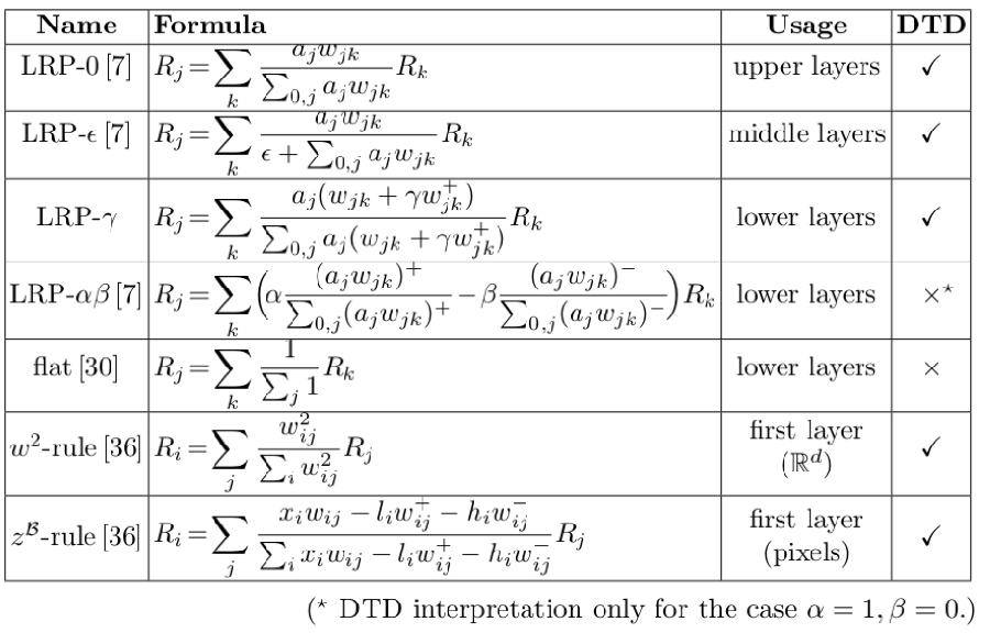
Relevance does not mean weight!! It is closely linked though. There are multiple possible Rules. These can be seen as "regularisations", mostly to reduce the noise/complexity of the produced explanations.

LRP-0: Basic
$z_{j} k$ = $w_{j} k * a_{j}$ , simply going backwards through the NN. Gives an explanation equivalent to Gradient * Input. This is undesirable because gradients are very noisy
LRP-𝟄: Epsilon
Add a small term $ϵ$ to the denominator. This aims to reduce the gradient noise by reducing the relevance of small contributions.
$R_{j} = \sum_{k} \frac{w_{j} k}{ϵ + \sum_{j} w_{j} k} R_{k}$ , notice the $ϵ$ at the denominator.
LRP-𝞬: Gamma
Try to improve stability by limiting how large positive or negative relevances can become. Adds a multiplication factor to $w_{j} k$ .
$R_{j} = \sum_{k} \frac{w_{j k} + γ * w_{j k}^{+}}{\sum_{j} w_{j k} + γ * w_{j k}^{+}} R_{k}$ , Notice the little plus above $w_{j k}^{+}$ . It signifies $a r g m a x (0, w_{j k})$
negative contributions get punished the higher $γ$ becomes. Small contributions get punished as well.

The explanation itself can be a heatmap of the pixels relevant for the activation of one output Neuron (class).

How to choose the right rule

LRP rules are set differently at different layers.

Pasted image 20240816150706.png

This was mostly found out via heuristic methods, but the results are actually based on deep taylor decomposition. Taylor decomposition simplifies each layer into the sum of functions that approximate it.

Example: why use LRP-0 in the upper layer:

Simplicity: These layers are very simple, and not subjected to the instability and interpretability issues of the lower layers. Therefore LRP-0 is sufficient.